| ORIGINAL VALUE | DESIRED VALUE | |||||||||||||||
| Tera | Giga | Mega | Myria | Kilo | Hecto | Deka | Basic Unit | Deci | Centi | Milla | Micro | Nano | Pico | Femto | Atto | |
| Tera | 3-> | 6-> | 8-> | 9-> | 10-> | 11-> | 12-> | 13-> | 14-> | 15-> | 18-> | 21-> | 24-> | 27-> | 30-> | |
| Giga | <-3 | 3-> | 5-> | 6-> | 7-> | 8-> | 9-> | 10-> | 11-> | 12-> | 15-> | 18-> | 21-> | 24-> | 27-> | |
| Mega | <-6 | <-3 | 2-> | 3-> | 4-> | 5-> | 6-> | 7-> | 8-> | 9-> | 12-> | 15-> | 18-> | 21-> | 24-> | |
| Myria | <-8 | <-5 | <-2 | 1-> | 2-> | 3-> | 4-> | 5-> | 6-> | 7-> | 10-> | 13-> | 16-> | 19-> | 22-> | |
| Kilo | <-9 | <-6 | <-3 | <-1 | 1-> | 2-> | 3-> | 4-> | 5-> | 6-> | 9-> | 12-> | 15-> | 18-> | 21-> | |
| Hecto | <-10 | <-7 | <-4 | <-2 | <-1 | 1-> | 2-> | 3-> | 4-> | 5-> | 8-> | 11-> | 14-> | 17-> | 20-> | |
| Deka | <-11 | <-8 | <-5 | <-3 | <-2 | <-1 | 1-> | 2-> | 3-> | 4-> | 7-> | 10-> | 13-> | 16-> | 19-> | |
| Basic Unit | <-12 | <-9 | <-6 | <-4 | <-3 | <-2 | <-1 | 1-> | 2-> | 3-> | 6-> | 9-> | 12-> | 15-> | 18-> | |
| Deci | <-13 | <-10 | <-7 | <-5 | <-4 | <-3 | <-2 | <-1 | 1-> | 2-> | 5-> | 8-> | 11-> | 14-> | 17-> | |
| Centi | <-14 | <-11 | <-8 | <-6 | <-5 | <-4 | <-3 | <-2 | <-1 | 1-> | 4-> | 7-> | 10-> | 13-> | 16-> | |
| Milli | <-15 | <-12 | <-9 | <-7 | <-6 | <-5 | <-4 | <-3 | <-2 | <-1 | 3-> | 6-> | 9-> | 12-> | 15-> | |
| Micro | <-18 | <-15 | <-12 | <-10 | <-9 | <-8 | <-7 | <-6 | <-5 | <-4 | <-3 | 3-> | 6-> | 9-> | 12-> | |
| Nano | <-21 | <-18 | <-15 | <-13 | <-12 | <-11 | <-10 | <-9 | <-8 | <-7 | <-6 | <-3 | 3-> | 6-> | 9-> | |
| Pico | <-24 | <-21 | <-18 | <-16 | <-15 | <-14 | <-13 | <-12 | <-11 | <-10 | <-9 | <-6 | <-3 | 3-> | 6-> | |
| Femto | <-27 | <-24 | <-21 | <-19 | <-18 | <-17 | <-16 | <-15 | <-14 | <-12 | <-10 | <-9 | <-6 | <-3 | 3-> | |
| Atto | <-30 | <-27 | <-24 | <-22 | <-21 | <-20 | <-19 | <-18 | <-17 | <-16 | <-15 | <-12 | <-9 | <-6 | <-3 | |
| The above metric conversion table provides a fast and automatic means of conversion from one metric notation to another. The term “Basic Unit” denotes the basic units of measurement, such as amperes, volts, ohms, watts, cycles, meters, grams, etc. To use the table, first locate the original or given value in the left-hand column. Now follow this line horizontally to the vertical column headed by the prefix of the desired value. The figure and arrow at this point indicates number of places and direction decimal point is to be moved. |
Example: Convert 0.15 ampere to milliamperes. Starting at the “Units” box in the left-hand column (since ampere is a basic unit of measurement), move horizontally to the column headed by the prefix “Milli,” and read 3->. Thus 0.15 ampere is the equivalent of 150 milliamperes. Example: Convert 50,000 kilocycles to megacycles. Read in the box horizontal to “kilo” and under “Mega,” the notation <-3, which means a shift of the decimal three places to the left. Thus 50,000 kilocycles is the equivalent of 50 megacycles. |
|||||||||||||||
- Categorie archieven ELECTRONICS DATA HANDBOOK
-
-
Metric Unit Prefixes
Prefix Symbol Power of 10 Numerical Value tera T 1012 trillion 1,000,000,000,000 1011 hundred-billion 100,000,000,000 1010 ten-billion 10,000,000,000 giga G 109 billion 1,000,000,000 108 hundred-million 100,000,000 107 ten-million 10,000,000 mega M 106 million 1,000,000 105 hundred-thousand 100,000 myria my 104 ten-thousand 10,000 kilo K 103 thousand 1,000 hecto h 102 hundred 100 deka 101 ten 10 100 one 1 deci d 10-1 tenth 0.1 centi c 10-2 hundredth 0.01 milli m 10-3 thousandth 0.001 10-4 ten-thousandth 0.000 1 10-5 hundred-thousandth 0.000 01 micro µ 10-6 millionth 0.000 001 10-7 ten-millionth 0.000 000 1 10-8 hundred-millionth 0.000 000 01 nano n 10-9 billionth 0.000 000 001 10-10 ten-billionth 0.000 000 000 1 10-11 hundred-billionth 0.000 000 000 01 pico p 10-12 trillionth 0.000 000 000 001 10-13 ten-trillionth 0.000 000 000 000 1 10-14 hundred-trillionth 0.000 000 000 000 01 femto f 10-15 quadrillionth 0.000 000 000 000 001 10-16 ten-quadrillionth 0.000 000 000 000 000 1 10-17 hundred-quadrillionth 0.000 000 000 000 000 01 atto a 10-18 ten-trillionth 0.000 000 000 000 000 001
-
Metric Relationships and New International Codes
Metric Relationships 
The above chart shows the relation of term watt is a basic unit). The number of the most used values in the American and
the metric systems of notation.steps so counted is three, and the direction
was to the left. Therefore, 5.0 milliwatts isthe equivalent of .005 watts. This chart also serves to quickly locate the decimal point in the conversion from
one metric expression to another.Example: Convert 5.0 milliwatts to watts.
Place the finger on milli and count the num-
ber of steps from there to units (since theExample: Convert 0.00035 microfarads to
picofarads (micromicrofarads). Here the
number of steps counted will be six to the
right. Therefore 0.00035 microfarads is the
equivalent of 350 picofarads.New International Codes The gradual adoption in this country of 2. “Kilomega” (km) has been replaced new international codes for metric prefixes by “giga” (G). amd measurement terminology by govern- “Hertz”. This term was recently adopted ment agencies, industry, technical maga-
zines, book publishers and others, is slowly
changing the system of measurement
and evaluation codes in general use
today.in the United States but it is not represented
in this handbook. It is, however, already
used by some publishers in place of”cycles”
in references to frequency specifications.The old familiar terms such as “cycles” (cyc), “kilocycles” (kc) and “megacycles” Acceptance of the new codes here, how- (Mc), are replaced by “Hertz” (Hz), ever, has been slow. We have , therefore,
continued to use the more familial termi-
nology in this handbook with the following
exceptions which appear in the metric“kilohertz” (kHz) and “megahertz”
(MHz).To combine two of these changes in one tables in the next two pages: specification, the old term “kilomegacycles”
(kMc) has become “gigahertz” (GHz).1. The cumbersome term “micromicro”
has been replaced by “pico”. Micro-
microfarad” (µµf) now becomes “pico-
farad” (pf).Heinrich Rudolph Hertz, was born in Germany in 1857 and died in 1894. He was
the first scientist to dect, create and
measure electromagnetic waves.
-
Single-Layer Wound Coil Chart
The chart on th opposite page provides a convenient
means of determining the unknown factors of small sized
single-layer wound r-f coils. Values thus found so cosely
approximate those determined by measurement or
mathematical calculation as to be entirely satisfactory
for all practical purposes of experimentation, design,
and repair work. Since in all coils of this type, the
difference between the mean and inner diameter of the
winding is so slight as to be negigible, D in all instances
may be either the mean or inner diameter as desired.
Example: Given the total number of turns, winding
length and diameter of a coil, — to find the inductance:
1. Place a straightedge on the chart so as to form
a line intersecting the number of turns N, and the
ratio of diameter to length K, and note the point
intersected on the linear axis column.2. Now move the straightedge so as to form a second line
which will intersect this same point on the axis column,
and the diameter D.
3. The point where this line intersects the L column indicates
the inductance of the coil in microhenries.Example: Given the diameter, winding length and inductance
in microhenries, — to find the number of turns;
1. Simply reverse the process outlined above for determining
inductance.
2. After finding the number of turns, consult the wire table on
page 35 and determine the size of the wire to be used.The dotted lines appearing on the chart illustrate the correct
ploting of a 600 microhenry coil consisting of 100 turns of wire
wound to 51/64″ on a form 2″ in diameter.Inductance, Capacitance, Reactance Charts
The direct-reading charts appearing on the following three
pages are designed for determining unknown values of
frequency, inductance, capacitance and reactance components
operating in a-f and r-f circuits.
The simplifications embodied in these charts make them
extremely useful. The frequency range covered comprises
the frequency spectrum from 1 cycle per second up to 1000
megacycles per second. All of the scales involved are plotted
in actual magnitudes so that no computations are required to
determine the location of the decimal point in the final result.
To make these conditions possible the frequency spectrum
has been divided into three parts:
Chart I (page 38)–Covers the range from 1 cycle to 1000
cycles.
Chart II (page 39)–From 1 kilocycle to 1000 kilocycles.
Chart III (page 40)–From 1 megacycle to 1000 megacycles.
Inductance, capacitance, reactance and frequency have been
plotted so that the reactance offered by an inductance at any
frequency may be readily determined by placing a straight-edge
across the chart connecting the know quantities.
Since XL = XC at resonance in most radio circuits, the chartsmay also be used to find the resonant frequency of any combi-
nation of L and C.To illustrate with a simple example, suppose the reactance
of a 0.01 uf. capacitor is desired at a frequency of 400 cycles.
Place a straight-edge across the proper chart so as to connect
the points 0.01 uf. and 400 cycles per sec. The quantity
desired is the point of intersection with the reactance scale
which is 40,000 ohms. The straight-edge also intersects the
inductance scale at 15.8 henrys indicating that this value of
inductance likewise has a reactance of 40,000 ohms at 400
cycles per sec. and furthermore, that these values of L and C
produce resonance at this frequency.There are many practical uses for these charts. The radio
experimentor, maintenance man and engineer will find them
helpful in the rapid solution of many reactance problems.
Unusual care was exercised in laying out the various scales
in order to secure a high degree of accuracy for the charts.
Results should be obatinable which are at least as accurate
as might be secured with a ten-inch slide rule.
-
Table of Standard Annealed Bare Copper Wire Using American Wire Gauge (B&S)
GAUGE DIAMETER INCHES AREA WEIGHT LENGTH RESISTANCE AT 68° F CURRENT CAPACITY (AWG) or (B&S) Min. Nom. Max. Circular Mils Pounds per M’ Feet per Lb. Ohms per M’ Feet per Ohm Ohms per Lb. (Amps) Rubber Insulated 0000 .4554 .4600 .4646 211600. 640.5 1.561 .04901 20400. .00007652 225 000 .4055 .4096 .4137 167800. 507.9 1.968 .06180 16180. .0001217 175 00 .3612 .3648 .3684 133100. 402.8 2.482 .07793 12830. .0001935 150 0 .3217 .3249 .3281 105500. 319.5 3.130 .09827 10180. .0003076 125 1 .2864 .2893 .2922 83690. 253.3 3.947 .1239 8070. .0004891 100 2 .2550 .2576 .2602 66370. 200.9 4.977 .1563 6400. .0007778 90 3 .2271 .2294 .2317 52640. 159.3 6.276 .1970 5075. .001237 80 4 .2023 .2043 .2063 41740. 126.4 7.914 .2485 4025. .001966 70 5 .1801 .1819 .1837 33100. 100.2 9.980 .3133 3192 .003127 55 6 .1604 .1620 .1636 26250. 79.46 12.58 .3951 2531. .004972 50 7 .1429 .1443 .1457 20820. 63.02 15.87 .4982 2007. .007905 – 8 .1272 .1285 .1298 16510. 49.98 20.01 .6282 1592. .01257 35 9 .1133 .1144 .1155 13090. 39.63 25.23 .7921 1262. .01999 – 10 .1009 .1019 .1029 10380. 31.43 31.82 .9989 1001. .03178 25 11 .08983 .09074 .09165 8234. 24.92 40.12 1.260 794. .05063 – 12 .08000 .08081 .08162 6530. 19.77 50.59 1.588 629.6 .08035 20 13 .07124 .07196 .07268 5178. 15.68 63.80 2.003 499.3 .1278 – 14 .06344 .06408 .06472 4107. 12.43 80.44 2.525 396.0 .2032 15 15 .05650 .05707 .05764 3257. 9.858 101.4 3.184 314.0 .3230 – 16 .05031 .05082 .05133 2583. 7.818 127.9 4.016 249.0 .5136 6 17 .04481 .04526 .04571 2048. 6.200 161.3 5.064 197.5 .8167 – 18 .03990 .04030 .04070 1624. 4.917 203.4 6.385 156.5 1.299 3 19 .03553 .03589 .03625 1288. 3.899 256.5 8.051 124.2 2.065 – 20 .03164 .03196 .03228 1022. 3.092 323.4 10.15 98.5 3.283 – 21 .02818 .02846 .02874 810.1 2.452 407.8 12.80 78.11 5.221 – 22 .02510 .02535 .02560 642.4 1.945 514.2 16.14 61.96 8.301 – 23 .02234 .02257 .02280 509.5 1.542 648.4 20.36 49.13 13.20 – 24 .01990 .02010 .02030 404.0 1.223 817.7 25.67 38.96 20.99 – 25 .01770 .01790 .01810 320.4 .9699 1031. 32.37 30.90 33.37 – 26 .01578 .01594 .01610 254.1 .7692 1300. 40.81 24.50 53.06 – 27 .01406 .01420 .01434 201.5 .6100 1639. 51.47 19.43 84.37 – 28 .01251 .01264 .01277 159.8 .4837 2067. 64.90 15.41 134.2 – 29 .01115 .01126 .01137 126.7 .3836 2607. 81.83 12.22 213.3 – 30 .00993 .01003 .01013 100.5 .3042 3287. 103.2 9.691 339.2 – 31 .008828 .008928 .009028 79.7 .2413 4145. 130.1 7.685 539.3 – 32 .007850 .007950 .008050 63.21 .1913 5227. 164.1 6.095 857.6 – 33 .006980 .007080 .007180 50.13 .1517 6591. 206.9 4.833 1364. – 34 .006205 .006305 .006405 39.75 .1203 8310. 260.9 3.833 2168. – 35 .005515 .005615 .005715 31.52 .09542 10480. 329.0 3.040 3448. – 36 .004900 .005000 .005100 25.00 .07568 13210. 414.8 2.411 5482. – 37 .004353 .004453 .004553 19.83 .06001 16660. 523.1 1.912 8717. – 38 .003865 .003965 .004065 15.72 .04759 21010. 659.6 1.516 13860. – 39 .003431 .003531 .003631 12.47 .03774 26500. 831.8 1.202 22040. – 40 .003045 .003145 .003245 9.888 .02993 33410. 1049. 0.9534 35040. – 41 .00270 .00280 .00290 7.8400 .02373 42140. 1323. .7559 55750. – 42 .00239 .00249 .00259 6.2001 .01877 53270. 1673. .5977 89120. – 43 .00212 .00222 .00232 4.9284 .01492 67020. 2104. .4753 141000. – 44 .00187 .00197 .00207 3.8809 .01175 85100. 2672. .3743 227380. – 45 .00166 .00176 .00186 3.0976 .00938 106600. 3348. .2987 356890. – 46 .00147 .00157 .00167 2.4649 .00746 134040. 4207. .2377 563900. – *Note: Values from National Electrical Code.
Note: per M’ means Per 1000 ft.
-
Coil Winding Data
Turns Per Inch Coil Winding Formulas Gauge (AWG) or (B&S) Number Of Turns per Linear Inch The following approximations for winding r-f coils are accurate to within approx. 1% for nearly all small air-core coils, where Enamel S.S.C. D.S.C. and S.C.C. D.C.C. 1 – – 3.3 3.3 L = self inductance in microhenrys
N = total number of turns
r = mean radius in inches
l= length of coil in inches
b = depth of coil in inches.2 – – 3.8 3.6 3 – – 4.2 4.0 4 – – 4.7 4.5 5 – – 5.2 5.0 single-Layer Wound Coils 6 – – 5.9 5.6 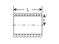
7 – – 6.5 6.2 8 7.6 – 7.4 7.1 9 8.6 – 8.2 7.8 10 9.6 – 9.3 8.9 11 10.7 – 10.3 9.8 12 12.0 – 11.5 10.9 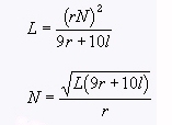
13 13.5 – 12.8 12.0 14 15.0 – 14.2 13.8 15 16.8 – 15.8 14.7 16 18.9 18.9 17.9 16.4 17 21.2 21.2 19.9 18.1 Multi-Layer Wound Coils 18 23.6 23.6 22.0 19.8 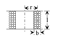
19 26.4 26.4 24.4 21.8 20 29.4 29.4 27.0 23.8 21 33.1 32.7 29.8 26.0 22 37.0 36.5 34.1 30.0 23 41.3 40.6 37.6 31.6 24 46.3 45.3 41.5 35.6 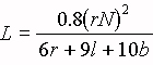
25 51.7 50.4 45.6 38.6 26 58.0 55.6 50.2 41.8 27 64.9 61.5 55.0 45.0 28 72.7 68.6 60.2 48.5 29 81.6 74.8 65.4 51.8 Spiral Wound Coils 30 90.5 83.3 71.5 55.5 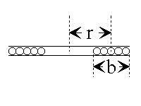
31 101. 92.0 77.5 59.2 32 113. 101. 83.6 62.6 33 127. 110. 90.3 66.3 34 143. 120. 97.0 70.0 35 158. 132. 104. 73.5 36 175. 143. 111. 77.0 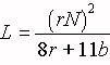
-
Ohm’s Law for A-C Circuits
The fundamental Ohm’s law formulas for
a-c circuits are given by:I = E / Z Z = E / I E = I*Z P = E*I*cos Ø Where: I = current in amperes, Z = impedance in Ohms, E = volts across, P = power in watts, Ø = phase angle in degrees. Phase Angle The phase angle is defined as the difference in degrees by which current leads voltage in a capacitive circuit, or lags voltage in an inductive circuit, and in series circuits is equal to the angle whose tangent is given by the ratio X/R and is expressed by: arc tan (X/R) Where: X = the inductive or capacitive reactance in ohms, R = the non-reactive resistance in ohms, of the combined resistive and reactive components of the circuit under consideration. Therefore: in a purely resistive circuit, Ø = 0° in a purely reactive circuit, Ø = 90° and in a resonant. circuit, Ø = 0° also when: Ø = 0°, cos Ø = l and P = E*I, Ø = 90°, cos Ø = 0 and P = 0. ————– Degrees x 0.0175 = radians.
1 radian = 57.3°Power Factor The power-factor of any a-c circuit is equal to
the true power in watts divided by the apparent
power in volt-amperes which is equal to the
cosine of the phase angle, and is expressed byE*I*cos Ø
p . f . = —————- = cos Ø
E*IWhere: p.f. = the circuit load power factor, E*I*cos Ø = the true power in watts, E*I* = the apparent power in voltamperes, E = the applied potential in volts I = load current in amperes. Therefore: in a purely resistive circuit. Ø = 0° and p.f. = 1 and in a reactive circuit, Ø = 90° and p.f. = 0 and in a resonant circuit, Ø = 0° and p.f. = 1 Ohm’s Law for D-C Circuits The fundamental Ohm’s law formulas for d-c circuits are given by, E
I = --- ,
RE
R = --- ,
IE = I*R P = I*E where: I = current in Amperes, R = resistance in ohms, E = potential across R in volts, P = power in watts. 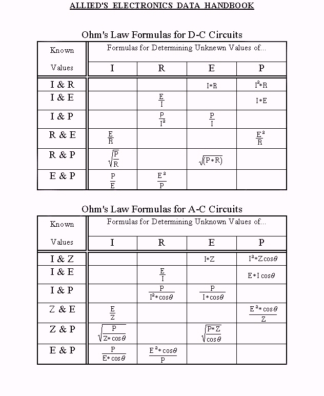
-
D-C Meter Formulas
Meter Resistance The d-c resistance of a milliameter or voltmeter movement may be determined as
follows:
1. Connect the meter in series with a
suitable battery and variable resist-
ance R1 as shown in the diagram above.2. Vary R1 until a full scale reading is
obtained.3. Connect another variable resistor R1
across the meter and vary its value
until a half scale reading is obtained.4. Disconnect R2 from the circuit and
measure its d-c resistance.The meter resistance RM is equal to the measured resistance of R2. Caution: Be sure that R1 has sufficient resistance to prevent an off scale reading
of the meter. The correct value depends
upon the sensitivity of meter, and voltage
of the battery. The following formula can
be used if the full scale current of the meter
is known:R1 = voltage of the battery used
full scale current of meter in amperes For safe results, use twice the value com-
puted. Also, never attempt to measure the
resistance of a meter with an ohmeter. To
do so would in all proability result in a
burned-out or severly damaged meter,
since the current required for the operation
of some ohmeters and bridges is far in
excess of the full scale current required by
the movement of the average meter you
may be checking.Ohms per Volt Rating of a Voltmeter 
Where: 
= ohms per volt, Ifs = full scale current in amperes. 

R = shunt value in ohms, N = the new full scale reading divided by the original full scale reading,
both being stated in the same units,RM = meter resistance in ohms Multi-Range Shunts 
R1 = intermediate or tapped shunt value in ohms, R1+2 = total resistance required for the low- est scale reading wanted, RM = meter resistance in ohms, N = the new full scale reading divided by the original full scale reading,
both being stated in the same units,Voltage Multipliers 
R = multiplier resistance in ohms, Efs = full scale reading required in volts, Ifs = full scale current of meter in am- peres, RM = meter resistance in ohms Measuring Resistance 
with Milliammeter and battery* 
RX = unknown resistance in ohms, RM = meter resistance in ohms, or effec- tive meter resistance if a shunted
range is used,I1 = current reading with switch open, I2 = current reading with switch closed, RL = current limiting resistor of suffi- cient value to keep meter reading
on scale when switch is open*Approximately true only when current limiting
resistor is large as compared to meter resistance.
FULL SCALE
CURRENTSHUNT
RESISTANCE0-10 ma
0-50 ma
0-100 ma
0-500 ma3.0 ohms
0.551 ohms
0.272 ohms
0.0541 ohmsMeasuring Resistance–(Continued) 
with Milliammeter, Battery and Known Resistor 
RX = unkown resistance in ohms, RY = kown resistance in ohms, RM = meter resistance in ohms, I1 = current reading with switch closed, I2 = current reading with switch open, 
with voltmeter and Battery 
RX = unkown resistance in ohms, RM = meter resistance in ohms, including multiplier resistance if a multiplied
range is used,E1 = voltmeter reading with switch closed, E2 = voltmeter reading with switch open,
FULL SCALE
VOLTAGEMULTIPLIER
RESISTANCE0-10 volts
0-50 volts
0-100 volts
0-250 volts
0-500 volts
0-1,000 volts10,000 ohms
50,000 ohms
100,000 ohms
250,000 ohms
500,000 ohms
1,000,000 ohms